9B. Sea Ice Supplementary
Explore the Sea Ice Data
![]()

![]()
![]()
Summary
In this notebook, we are going to explore the dataset used for the PMP Sea Ice demo notebook. Let’s explore the sea ice data for fun!
Notebook Authors: Jiwoo Lee, Ana Ordonez, Paul Durack, Peter Gleckler (PCMDI, Lawrence Livermore National Laboratory)
Table of Contents
Note: Links to the sections work best when viewing this notebook via nbviewer.
1. Environment setup
2. Model Data
2.1 Load data
2.1.1 Open dataset
2.1.2 Visualize the data
2.2 Sea ice extent
3. Reference Data
3.1 Load data
3.1.1 Open Reference Dataset for Arctic
3.1.2 Open Reference Dataset for Antartica
3.2 Sea ice extent
4. Diagnostics: Climatology Annual Cycle
5. Evaluation Metrics
5.1 Mean Square Error (Annual Mean)
5.2 Temporal Mean Square Error (Annual Cycle)
1. Environment setup
We will use multiple libraries for this analysis.
xCDAT: an open source Python tool built to make climate data analysis easy. xCDAT is an extension of xarray for data analysis on structured grids.
numpy: a dependency required to manage n-dimensional array data.
matplotlib and cartopy: required for data visualization.
[1]:
import xcdat as xc
import numpy as np
import matplotlib.pyplot as plt
import cartopy.crs as ccrs
Go back to Top
2. Model Data
2.1 Load data
2.1.1 Open dataset
This demo uses one of the numerous CMIP6 models – E3SM-1-0. The Sea-Ice Area Percentage (Ocean Grid; ‘siconc’) and Grid-Cell Area for Ocean Variables (‘areacello’) variables are needed and can be found in the directories listed below. In addition, six other models are available that can augment the analyses in this demo:
/p/user_pub/pmp/demo/sea-ice/links_siconc
/p/user_pub/pmp/demo/sea-ice/links_area
This data can be found from ESGF (https://esgf-node.llnl.gov/).
e.g., Search query: https://aims2.llnl.gov/search?project=CMIP6&activeFacets={“experiment_id”:”historical”,”variable_id”:”siconc”}
Go back to Top
[2]:
!ls demo_data/CMIP5_demo_timeseries/historical/ice/mon/siconc_SImon_E3SM-1-0_historical_r1i1p1f1_gr_201001-201412.nc
demo_data/CMIP5_demo_timeseries/historical/ice/mon/siconc_SImon_E3SM-1-0_historical_r1i1p1f1_gr_201001-201412.nc
[3]:
!ls demo_data/misc_demo_data/fx/areacello_Ofx_E3SM-1-0_historical_r1i1p1f1_gr.nc
demo_data/misc_demo_data/fx/areacello_Ofx_E3SM-1-0_historical_r1i1p1f1_gr.nc
[4]:
# Load model dataset
ds = xc.open_mfdataset(
    "demo_data/CMIP5_demo_timeseries/historical/ice/mon/siconc_SImon_E3SM-1-0_historical_r1i1p1f1_gr_201001-201412.nc"
)
area = xc.open_dataset(
    "demo_data/misc_demo_data/fx/areacello_Ofx_E3SM-1-0_historical_r1i1p1f1_gr.nc"
)
2026-05-24 14:55:26,217 [WARNING]: dataset.py(open_dataset:121) >> "No time coordinates were found in this dataset to decode. If time coordinates were expected to exist, make sure they are detectable by setting the CF 'axis' or 'standard_name' attribute (e.g., ds['time'].attrs['axis'] = 'T' or ds['time'].attrs['standard_name'] = 'time'). Afterwards, try decoding again with `xcdat.decode_time`."
See what is in the dataset:
[5]:
ds
[5]:
<xarray.Dataset> Size: 16MB
Dimensions:    (time: 60, bnds: 2, lat: 180, lon: 360)
Coordinates:
  * time       (time) object 480B 2010-01-16 12:00:00 ... 2014-12-16 12:00:00
  * lat        (lat) float64 1kB -89.5 -88.5 -87.5 -86.5 ... 86.5 87.5 88.5 89.5
  * lon        (lon) float64 3kB 0.5 1.5 2.5 3.5 4.5 ... 356.5 357.5 358.5 359.5
    type       |S7 7B ...
Dimensions without coordinates: bnds
Data variables:
    time_bnds  (time, bnds) object 960B dask.array<chunksize=(1, 2), meta=np.ndarray>
    lat_bnds   (lat, bnds) float64 3kB dask.array<chunksize=(180, 2), meta=np.ndarray>
    lon_bnds   (lon, bnds) float64 6kB dask.array<chunksize=(360, 2), meta=np.ndarray>
    siconc     (time, lat, lon) float32 16MB dask.array<chunksize=(1, 180, 360), meta=np.ndarray>
Attributes: (12/46)
    Conventions:            CF-1.7 CMIP-6.2
    activity_id:            CMIP
    branch_method:          standard
    branch_time_in_child:   0.0
    branch_time_in_parent:  36500.0
    contact:                Dave Bader (bader2@llnl.gov)
    ...                     ...
    title:                  E3SM-1-0 output prepared for CMIP6
    tracking_id:            hdl:21.14100/cdef87ba-4537-408d-8818-63da6fee1409
    variable_id:            siconc
    variant_label:          r1i1p1f1
    license:                CMIP6 model data produced by E3SM is licensed und...
cmor_version: 3.4.0[6]:
area
[6]:
<xarray.Dataset> Size: 272kB
Dimensions:    (lat: 180, bnds: 2, lon: 360)
Coordinates:
  * lat        (lat) float64 1kB -89.5 -88.5 -87.5 -86.5 ... 86.5 87.5 88.5 89.5
  * lon        (lon) float64 3kB 0.5 1.5 2.5 3.5 4.5 ... 356.5 357.5 358.5 359.5
Dimensions without coordinates: bnds
Data variables:
    lat_bnds   (lat, bnds) float64 3kB ...
    lon_bnds   (lon, bnds) float64 6kB ...
    areacello  (lat, lon) float32 259kB ...
Attributes: (12/46)
    Conventions:            CF-1.7 CMIP-6.2
    activity_id:            CMIP
    branch_method:          standard
    branch_time_in_child:   0.0
    branch_time_in_parent:  36500.0
    creation_date:          2021-01-28T04:40:15Z
    ...                     ...
    title:                  E3SM-1-0 output prepared for CMIP6
    tracking_id:            hdl:21.14100/aaa3a5b2-c4c4-4bf6-b7a3-b59915926fc0
    variable_id:            areacello
    variant_label:          r1i1p1f1
    license:                CMIP6 model data produced by E3SM is licensed und...
cmor_version: 3.6.0Go back to Top
2.1.2 Visualize the data
Go back to Top
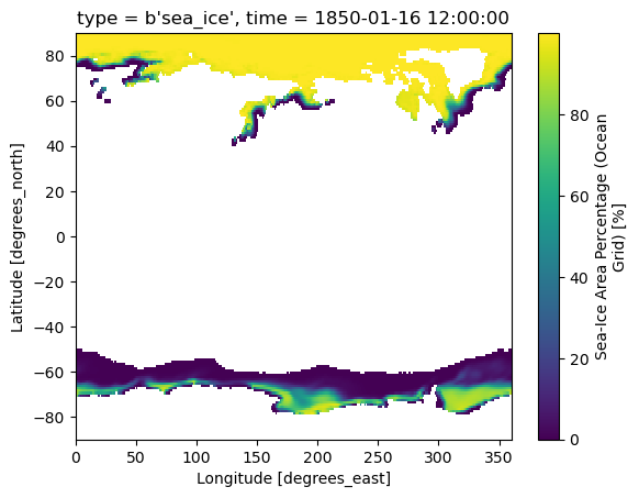
a. Quick look
Let’s take a quick look at a single timestep of the data:
[7]:
ds["siconc"].isel(time=0).plot()
[7]:
<matplotlib.collections.QuadMesh at 0x1bf467200>
[8]:
ds["siconc"].isel(time=0).to_numpy()
[8]:
array([[      nan,       nan,       nan, ...,       nan,       nan,
              nan],
       [      nan,       nan,       nan, ...,       nan,       nan,
              nan],
       [      nan,       nan,       nan, ...,       nan,       nan,
              nan],
       ...,
       [99.499756, 99.51926 , 99.52034 , ..., 99.43246 , 99.441185,
        99.46285 ],
       [99.60115 , 99.60065 , 99.59965 , ..., 99.5979  , 99.60229 ,
        99.60173 ],
       [99.68882 , 99.66776 , 99.63899 , ..., 99.71866 , 99.709045,
        99.69889 ]], shape=(180, 360), dtype=float32)
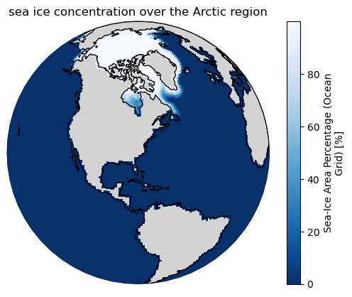
b. Snapshot on map
Viewing the same data from another angle:
Example mapping scripts are adapted and revised from https://docs.xarray.dev/en/latest/user-guide/plotting.html#maps.
Go back to Top
[9]:
from cartopy.feature import LAND as cartopy_land
from cartopy.feature import OCEAN as cartopy_ocean
[10]:
ax = plt.axes(projection=ccrs.Orthographic(-80, 35))

ax.set_global()

# Color over the ocean
ax.add_feature(cartopy_ocean, zorder=1, edgecolor="none", facecolor="lightblue")

# Data
ds["siconc"].isel(time=0).plot.pcolormesh(ax=ax, transform=ccrs.PlateCarree(), cmap="Blues_r", zorder=3)

# Color over the land
ax.add_feature(cartopy_land, zorder=2, edgecolor="k", facecolor="lightgrey")

# Add coastlines
ax.coastlines(color="black", zorder=4)

ax.set_title("sea ice concentration over the Arctic region")
[10]:
Text(0.5, 1.0, 'sea ice concentration over the Arctic region')
/Users/lee1043/miniforge3/envs/pmp_devel_20260331/lib/python3.12/site-packages/shapely/creation.py:730: RuntimeWarning: invalid value encountered in create_collection
  return lib.create_collection(geometries, np.intc(typ), out=out, **kwargs)
/Users/lee1043/miniforge3/envs/pmp_devel_20260331/lib/python3.12/site-packages/shapely/creation.py:730: RuntimeWarning: invalid value encountered in create_collection
  return lib.create_collection(geometries, np.intc(typ), out=out, **kwargs)
/Users/lee1043/miniforge3/envs/pmp_devel_20260331/lib/python3.12/site-packages/shapely/creation.py:730: RuntimeWarning: invalid value encountered in create_collection
  return lib.create_collection(geometries, np.intc(typ), out=out, **kwargs)
/Users/lee1043/miniforge3/envs/pmp_devel_20260331/lib/python3.12/site-packages/shapely/creation.py:730: RuntimeWarning: invalid value encountered in create_collection
  return lib.create_collection(geometries, np.intc(typ), out=out, **kwargs)
/Users/lee1043/miniforge3/envs/pmp_devel_20260331/lib/python3.12/site-packages/shapely/creation.py:730: RuntimeWarning: invalid value encountered in create_collection
  return lib.create_collection(geometries, np.intc(typ), out=out, **kwargs)
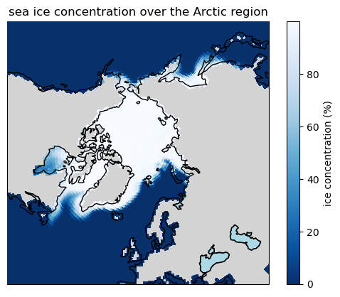
Let’s plot the data using another angle, zooming in on the Arctic region:
Additional matplotlib colorshemes can be found here.
[11]:
# Generate a map
proj = ccrs.NorthPolarStereo()
ax = plt.subplot(111, projection=proj)
ax.set_global()

# Color over the ocean
ax.add_feature(cartopy_ocean, zorder=1, edgecolor="none", facecolor="lightblue")

# Color over the land
ax.add_feature(cartopy_land, zorder=2, edgecolor="k", facecolor="lightgrey")

# Data
ds["siconc"].isel(time=0).plot.pcolormesh(
    ax=ax,
    x="lon",
    y="lat",
    transform=ccrs.PlateCarree(),
    cmap="Blues_r",
    cbar_kwargs={"label": "ice concentration (%)"},
    zorder=3,
)

# Add coastlines
ax.coastlines(color="black", zorder=4)

ax.set_extent([-180, 180, 43, 90], ccrs.PlateCarree())
ax.set_title("sea ice concentration over the Arctic region")
[11]:
Text(0.5, 1.0, 'sea ice concentration over the Arctic region')
/Users/lee1043/miniforge3/envs/pmp_devel_20260331/lib/python3.12/site-packages/shapely/creation.py:730: RuntimeWarning: invalid value encountered in create_collection
  return lib.create_collection(geometries, np.intc(typ), out=out, **kwargs)
/Users/lee1043/miniforge3/envs/pmp_devel_20260331/lib/python3.12/site-packages/shapely/creation.py:730: RuntimeWarning: invalid value encountered in create_collection
  return lib.create_collection(geometries, np.intc(typ), out=out, **kwargs)
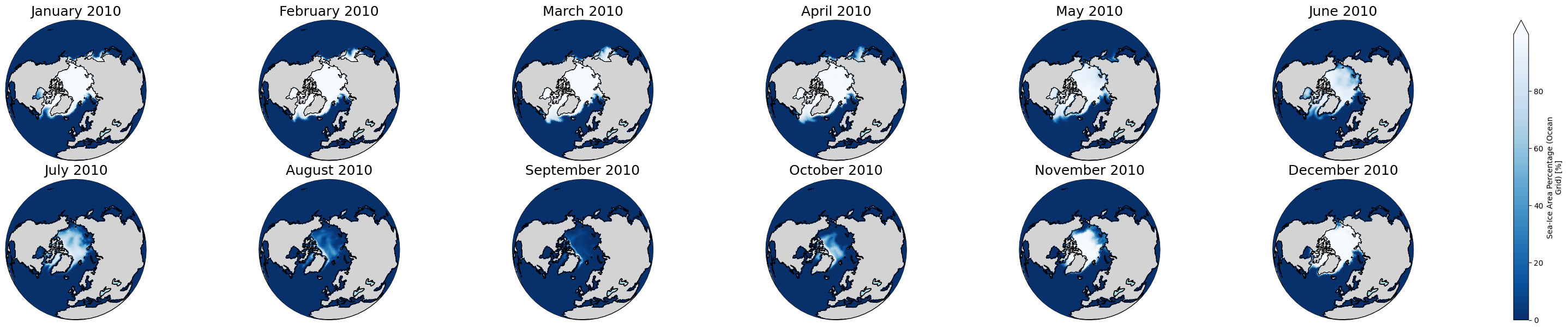
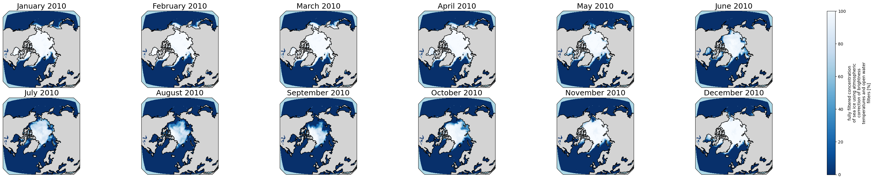
c. See the data evolving in time
Arctic:
Go back to Top
[12]:
proj_plot = ccrs.Orthographic(0, 90)

years_to_show = [2010]  # You can edit this to check another year(s). It could include multiple years, e.g., [2010, 2011, 2012]


p = ds['siconc'].sel(time = ds.time.dt.year.isin(years_to_show)).plot(x='lon', y='lat',
                                                                 transform=ccrs.PlateCarree(),
                                                                 aspect=ds.sizes["lon"] / ds.sizes["lat"],  # for a sensible figsize
                                                                 subplot_kws={"projection": proj_plot},
                                                                 col='time', col_wrap=6, robust=True, cmap='Blues_r', zorder=3)

# We have to set the map's options on all four axes
for ax,i in zip(p.axs.flat,  ds.time.sel(time = ds.time.dt.year.isin(years_to_show)).values):
    ax.set_title(i.strftime("%B %Y"), fontsize=18)
    # Color over the ocean
    ax.add_feature(cartopy_ocean, zorder=1, edgecolor="none", facecolor="lightblue")
    # Color over the land
    ax.add_feature(cartopy_land, zorder=2, edgecolor="k", facecolor="lightgrey")
    # Draw coastlines
    ax.coastlines(zorder=4)
/Users/lee1043/miniforge3/envs/pmp_devel_20260331/lib/python3.12/site-packages/shapely/creation.py:730: RuntimeWarning: invalid value encountered in create_collection
  return lib.create_collection(geometries, np.intc(typ), out=out, **kwargs)
/Users/lee1043/miniforge3/envs/pmp_devel_20260331/lib/python3.12/site-packages/shapely/creation.py:730: RuntimeWarning: invalid value encountered in create_collection
  return lib.create_collection(geometries, np.intc(typ), out=out, **kwargs)
/Users/lee1043/miniforge3/envs/pmp_devel_20260331/lib/python3.12/site-packages/shapely/creation.py:730: RuntimeWarning: invalid value encountered in create_collection
  return lib.create_collection(geometries, np.intc(typ), out=out, **kwargs)
/Users/lee1043/miniforge3/envs/pmp_devel_20260331/lib/python3.12/site-packages/shapely/creation.py:730: RuntimeWarning: invalid value encountered in create_collection
  return lib.create_collection(geometries, np.intc(typ), out=out, **kwargs)
Go back to Top
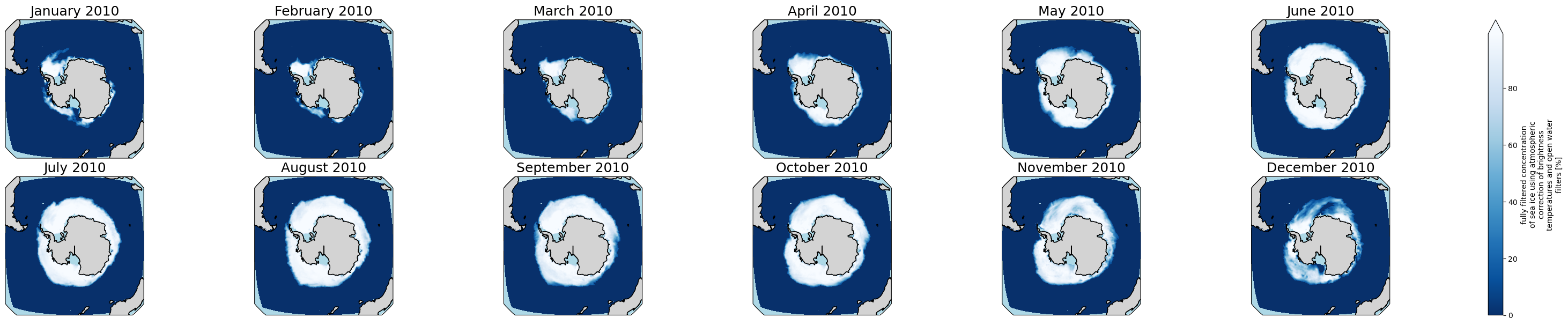
Antartic:
[13]:
proj_plot = ccrs.Orthographic(0, -90)

#years_to_show = [2010]  # You can uncomment and edit this to check another year(s). It could include multiple years, e.g., [2010, 2011, 2012]

p = ds['siconc'].sel(time = ds.time.dt.year.isin(years_to_show)).plot(x='lon', y='lat',
                                                                 transform=ccrs.PlateCarree(),
                                                                 aspect=ds.sizes["lon"] / ds.sizes["lat"],  # for a sensible figsize
                                                                 subplot_kws={"projection": proj_plot},
                                                                 col='time', col_wrap=6, robust=True, cmap='Blues_r', zorder=3)

# We have to set the map's options on all four axes
for ax,i in zip(p.axs.flat,  ds.time.sel(time = ds.time.dt.year.isin(years_to_show)).values):
    ax.set_title(i.strftime("%B %Y"), fontsize=18)
    # Color over the ocean
    ax.add_feature(cartopy_ocean, zorder=1, edgecolor="none", facecolor="lightblue")
    # Color over the land
    ax.add_feature(cartopy_land, zorder=2, edgecolor="k", facecolor="lightgrey")
    # Draw coastlines
    ax.coastlines(zorder=4)
/Users/lee1043/miniforge3/envs/pmp_devel_20260331/lib/python3.12/site-packages/shapely/creation.py:730: RuntimeWarning: invalid value encountered in create_collection
  return lib.create_collection(geometries, np.intc(typ), out=out, **kwargs)
/Users/lee1043/miniforge3/envs/pmp_devel_20260331/lib/python3.12/site-packages/shapely/creation.py:730: RuntimeWarning: invalid value encountered in create_collection
  return lib.create_collection(geometries, np.intc(typ), out=out, **kwargs)

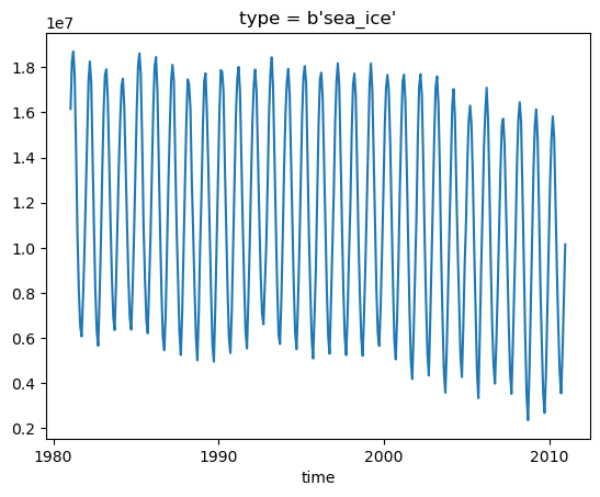
2.2 Sea ice extent
Go back to Top
Below, we will calculate the sea ice extent from sea ice concentration.
[14]:
sea_ice_extent = (ds.siconc.where(ds.lat > 0) * 1e-2 * area.areacello * 1e-6).where(ds.siconc > 15).sum(("lat", "lon"))
Note for the above line
where siconc > 15: to consider sea ice extent instead of total sea ice area
multiply 1e-2: to convert percentage (%) to fraction
To learn more about the sea ice extent, see this article from NSIDC.
Go back to Top
Visualize the sea ice extent time series:
[15]:
sea_ice_extent.sel({"time": slice("2010-01-01", "2014-12-31")}).plot()
[15]:
[<matplotlib.lines.Line2D at 0x1bfa257f0>]
Let’s add the sea_ice_extent dataArray to the dataset (ds) for later use:
[16]:
ds["extent"] = sea_ice_extent
[17]:
ds
[17]:
<xarray.Dataset> Size: 16MB
Dimensions:    (time: 60, bnds: 2, lat: 180, lon: 360)
Coordinates:
  * time       (time) object 480B 2010-01-16 12:00:00 ... 2014-12-16 12:00:00
  * lat        (lat) float64 1kB -89.5 -88.5 -87.5 -86.5 ... 86.5 87.5 88.5 89.5
  * lon        (lon) float64 3kB 0.5 1.5 2.5 3.5 4.5 ... 356.5 357.5 358.5 359.5
    type       |S7 7B ...
Dimensions without coordinates: bnds
Data variables:
    time_bnds  (time, bnds) object 960B dask.array<chunksize=(1, 2), meta=np.ndarray>
    lat_bnds   (lat, bnds) float64 3kB dask.array<chunksize=(180, 2), meta=np.ndarray>
    lon_bnds   (lon, bnds) float64 6kB dask.array<chunksize=(360, 2), meta=np.ndarray>
    siconc     (time, lat, lon) float32 16MB dask.array<chunksize=(1, 180, 360), meta=np.ndarray>
    extent     (time) float32 240B dask.array<chunksize=(1,), meta=np.ndarray>
Attributes: (12/46)
    Conventions:            CF-1.7 CMIP-6.2
    activity_id:            CMIP
    branch_method:          standard
    branch_time_in_child:   0.0
    branch_time_in_parent:  36500.0
    contact:                Dave Bader (bader2@llnl.gov)
    ...                     ...
    title:                  E3SM-1-0 output prepared for CMIP6
    tracking_id:            hdl:21.14100/cdef87ba-4537-408d-8818-63da6fee1409
    variable_id:            siconc
    variant_label:          r1i1p1f1
    license:                CMIP6 model data produced by E3SM is licensed und...
cmor_version: 3.4.0Go back to Top
3. Reference Data
The observational dataset provided is the satellite derived sea ice concentration dataset from EUMETSAT OSI-SAF. More data information can be found at the osi-450-a product page. The path to this data is:
/p/user_pub/pmp/demo/sea-ice/EUMETSAT
This data can be also downloaded via the PMP’s Demo #0 notebook.
3.1 Load data
3.1.1 Open Reference Dataset for Arctic
Go back to Top
[18]:
obs_file1 = "demo_data/misc_demo_data/ocn/ice_conc_nh_ease2-250_cdr-v3p0_198801-202012.nc"
obs_ds = xc.open_dataset(obs_file1)
2026-05-24 14:55:32,238 [WARNING]: bounds.py(add_missing_bounds:192) >> The yc coord variable has a 'units' attribute that is not in degrees.
[19]:
obs_ds
[19]:
<xarray.Dataset> Size: 1GB
Dimensions:                 (time: 396, yc: 432, xc: 432, nv: 2, bnds: 2)
Coordinates:
  * time                    (time) object 3kB 1988-01-16 12:00:00 ... 2020-12...
  * yc                      (yc) float64 3kB 5.388e+03 5.362e+03 ... -5.388e+03
  * xc                      (xc) float64 3kB -5.388e+03 -5.362e+03 ... 5.388e+03
    lat                     (yc, xc) float32 746kB ...
    lon                     (yc, xc) float32 746kB ...
Dimensions without coordinates: nv, bnds
Data variables:
    Lambert_Azimuthal_Grid  int32 4B ...
    ice_conc                (time, yc, xc) float64 591MB ...
    raw_ice_conc_values     (time, yc, xc) float64 591MB ...
    status_flag             (time, yc, xc) float32 296MB ...
    time_bnds               (time, nv) object 6kB ...
    xc_bnds                 (xc, bnds) float64 7kB ...
Attributes: (12/43)
    title:                     Monthly Sea Ice Concentration Climate Data Rec...
    summary:                   This climate data record of sea ice concentrat...
    topiccategory:             Oceans ClimatologyMeteorologyAtmosphere
    geospatial_lat_min:        16.62393
    geospatial_lat_max:        90.0
    geospatial_lon_min:        -180.0
    ...                        ...
    algorithm:                 SICCI3LF (19V, 37V, 37H)
    references:                Product User Manual v3 (2022),Algorithm Theore...
    contributor_name:          Thomas Lavergne,Atle Soerensen,Rasmus Tonboe,C...
    contributor_role:          PrincipalInvestigator,author,author,author,aut...
    source:                    FCDR of SMMR / SSMI / SSMIS Brightness Tempera...
product_status: released[20]:
proj_plot = ccrs.Orthographic(0, 90)

#years_to_show = [2000]  # You can uncomment and edit this to check another year(s). It could include multiple years, e.g., [2000, 2001, 2002]

p = obs_ds['ice_conc'].sel(time = obs_ds.time.dt.year.isin(years_to_show)).plot(x='lon', y='lat',
                                                                 transform=ccrs.PlateCarree(),
                                                                 aspect=ds.dims["lon"] / ds.dims["lat"],  # for a sensible figsize
                                                                 subplot_kws={"projection": proj_plot},
                                                                 col='time', col_wrap=6, robust=True, cmap='Blues_r', zorder=3)

# We have to set the map's options on all four axes
for ax,i in zip(p.axs.flat,  ds.time.sel(time = ds.time.dt.year.isin(years_to_show)).values):
    ax.set_title(i.strftime("%B %Y"), fontsize=18)
    # Color over the ocean
    ax.add_feature(cartopy_ocean, zorder=1, edgecolor="none", facecolor="lightblue")
    # Color over the land
    ax.add_feature(cartopy_land, zorder=2, edgecolor="k", facecolor="lightgrey")
    # Draw coastlines
    ax.coastlines(zorder=4)
/var/folders/wh/jt7ywcnn01z8xcrr1p_dzp8r001rcz/T/ipykernel_32547/56113352.py:7: FutureWarning: The return type of `Dataset.dims` will be changed to return a set of dimension names in future, in order to be more consistent with `DataArray.dims`. To access a mapping from dimension names to lengths, please use `Dataset.sizes`.
  aspect=ds.dims["lon"] / ds.dims["lat"],  # for a sensible figsize
Go back to Top
3.1.2 Open Reference Dataset for Antartica
Go back to Top
[21]:
obs_file2 = "demo_data/misc_demo_data/ocn/ice_conc_sh_ease2-250_cdr-v3p0_198801-202012.nc"
obs_ds2 = xc.open_dataset(obs_file2)
2026-05-24 14:55:36,335 [WARNING]: bounds.py(add_missing_bounds:192) >> The yc coord variable has a 'units' attribute that is not in degrees.
[22]:
proj_plot = ccrs.Orthographic(0, -90)

#years_to_show = [2000]  # You can uncomment and edit this to check another year(s). It could include multiple years, e.g., [2000, 2001, 2002]

p = obs_ds2['ice_conc'].sel(time = obs_ds2.time.dt.year.isin(years_to_show)).plot(x='lon', y='lat',
                                                                 transform=ccrs.PlateCarree(),
                                                                 aspect=ds.dims["lon"] / ds.dims["lat"],  # for a sensible figsize
                                                                 subplot_kws={"projection": proj_plot},
                                                                 col='time', col_wrap=6, robust=True, cmap='Blues_r', zorder=3)

# We have to set the map's options on all four axes
for ax,i in zip(p.axs.flat,  ds.time.sel(time = ds.time.dt.year.isin(years_to_show)).values):
    ax.set_title(i.strftime("%B %Y"), fontsize=18)
    # Color over the ocean
    ax.add_feature(cartopy_ocean, zorder=1, edgecolor="none", facecolor="lightblue")
    # Color over the land
    ax.add_feature(cartopy_land, zorder=2, edgecolor="k", facecolor="lightgrey")
    # Draw coastlines
    ax.coastlines(zorder=4)
/var/folders/wh/jt7ywcnn01z8xcrr1p_dzp8r001rcz/T/ipykernel_32547/1061999368.py:7: FutureWarning: The return type of `Dataset.dims` will be changed to return a set of dimension names in future, in order to be more consistent with `DataArray.dims`. To access a mapping from dimension names to lengths, please use `Dataset.sizes`.
  aspect=ds.dims["lon"] / ds.dims["lat"],  # for a sensible figsize
3.2 Sea ice extent
Go back to Top
[23]:
obs_area = 625
obs_sea_ice_extent = (obs_ds.ice_conc.where(obs_ds.lat > 0).where(obs_ds.ice_conc > 15) * 1e-2 * obs_area).sum(("xc", "yc"))
Note for the above lines
obs_area = 625 # area size represented by each grid (625 km^2 = 25 km x 25 km resolution)
where ice_conc > 15: to consider sea ice extent instead of total sea ice area
multiply 1e-2: to convert percentage (%) to fraction
[24]:
obs_sea_ice_extent.plot()
[24]:
[<matplotlib.lines.Line2D at 0x1c0037200>]
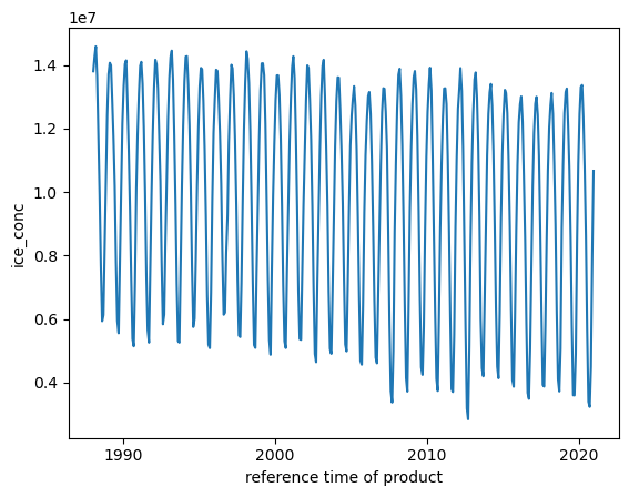
Let’s add the obs_arctic dataArray to the dataset (obs_ds) for later use:
[25]:
obs_ds["extent"] = obs_sea_ice_extent
Go back to Top
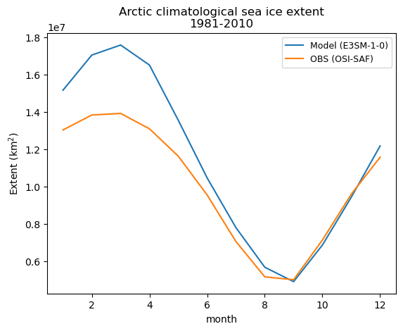
4. Diagnostics: Climatology Annual Cycle
Let’s analyze the climatology of Sea-Ice extent, focusing on its annual cycle.
We will use xCDAT’s `temporal.climatology <https://xcdat.readthedocs.io/en/latest/generated/xarray.Dataset.temporal.climatology.html>`__ function to calculate the monthly climatology field.
Go back to Top
[26]:
obs_ds_clim = obs_ds.temporal.climatology(
    "extent", freq="month", reference_period=("2010-01-01", "2014-12-31"))
[27]:
ds_clim = ds.temporal.climatology(
    "extent", freq="month", reference_period=("2010-01-01", "2014-12-31"))
[28]:
fig, ax = plt.subplots()

# Unify the time axis to plot lines on a same figure
ds_clim["time"] = [x for x in range(1, 13)]
obs_ds_clim["time"] = [x for x in range(1, 13)]

# Add lines
ds_clim["extent"].plot(ax=ax, label="Model (E3SM-1-0)")
obs_ds_clim["extent"].plot(ax=ax, label="OBS (OSI-SAF)")

# Attach legend
plt.title("Arctic climatological sea ice extent\n1981-2010")
plt.xlabel("month")
plt.ylabel("Extent (km${^2}$)")
plt.legend(loc="upper right", fontsize=9)
[28]:
<matplotlib.legend.Legend at 0x1c0379a30>
Go back to Top
5. Evaluation Metrics
The term “metric” indicates a score or statistics that can represent a model’s performance in reproducing observed features. A “metric” can be defined in many different ways, but the primary purpose of metrics is to summarize the performances of many different models and provide a framework for benchmarking model realism.
In this notebook, we define Mean Square Error (MSE) and Temporal MSE as metrics.
5.1 Mean Square Error (Annual Mean)
Go back to Top
[29]:
mse = (ds_clim["extent"].data.mean() - obs_ds_clim["extent"].data.mean()) ** 2 * 1e-12
[30]:
print(f"Mean Square Error: {float(mse)} 10^12 km^4")
Mean Square Error: 0.22072134548040453 10^12 km^4
5.2 Temporal Mean Square Error (Annual Cycle)
Go back to Top
[31]:
tmse = np.sum(((ds_clim["extent"].data - obs_ds_clim["extent"].data) ** 2)) / len(ds_clim["extent"]) * 1e-12
[32]:
print(f"Temporal Mean Square Error: {float(tmse)} 10^12 km^4")
Temporal Mean Square Error: 1.6153168220537057 10^12 km^4
Go back to Top